Read PDB structures from the database and generate NERDSS inputs
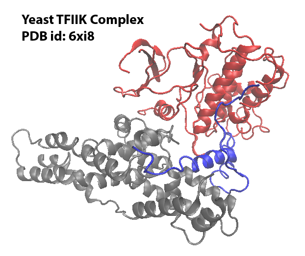
This tutorial will explore how to generate inputs for NERDSS using the real PDB structure with the Yeast TFIIK Complex as an example. Download the PDB file and save it under your working directory.
Install and Import the library
pip install ioNERDSS
import ioNERDSS as ion
Visualize the PDB structure
This PDB structure has 3 chains. Each chain will be modeled to a molecule type in NERDSS simulation. And the molecules can assemble into the complex.
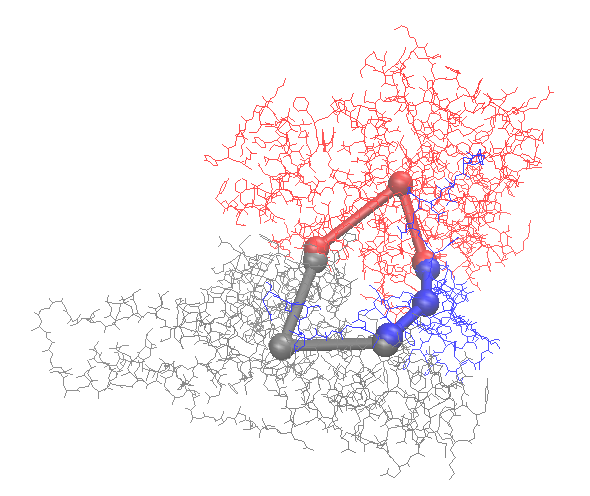
Use ioNERDSS to construct the coarse-grained structure
ion.cg('6xi8', 3.5)
The coarse-graind structure is saved as output.pdb. Following is the visualization of the original structure and the coarse-grained structure:
The output for NERDSS input structure parameters:
COM of chain C: 8.560, 9.803, 10.088
Interfaces of chain C: CA partner chain: A 8.936 10.472 9.434 energy: 91.000
CB partner chain: B 8.827 9.069 10.649 energy: 100.310

COM of chain A: 9.204, 10.077, 7.857
Interfaces of chain A: AC partner chain: C 9.016 10.492 9.302 energy: 91.000
AB partner chain: B 10.524 9.176 8.997 energy: 61.450

COM of chain B: 10.686, 8.405, 10.765
Interfaces of chain B: BC partner chain: C 8.893 9.041 10.748 energy: 100.310
BA partner chain: A 10.544 9.154 9.213 energy: 61.450

output.pdb has been generated.
nerdss input parameters:
mol C:
  com 0.000 0.000 0.000
  CA [0.376, 0.669, -0.654]
      partner A
      partner interface: AC
      theta1 2.548 theta2 2.563 phi1 -0.749 phi2 1.886 omega 0.808
      [2.548, 2.563, -0.749, 1.886, 0.808]
      n1 0.000 0.000 1.000
      n2 0.000 0.000 1.000
       sigma 0.156
       energy 91.000
  CB [0.267, -0.733, 0.560]
      partner B
      partner interface: BC
      theta1 2.496 theta2 2.205 phi1 2.351 phi2 -0.047 omega -1.672
      [2.496, 2.205, 2.351, -0.047, -1.672]
      n1 0.000 0.000 1.000
      n2 0.000 0.000 1.000
       sigma 0.122
       energy 100.310
mol A:
  com 0.000 0.000 0.000
  AC [-0.188, 0.415, 1.446]
      partner C
      partner interface: CA
      theta1 2.563 theta2 2.548 phi1 1.886 phi2 -0.749 omega 0.808
      [2.563, 2.548, 1.886, -0.749, 0.808]
      n1 0.000 0.000 1.000
      n2 0.000 0.000 1.000
       sigma 0.156
       energy 91.000
  AB [1.320, -0.900, 1.141]
      partner B
      partner interface: BA
      theta1 2.327 theta2 2.797 phi1 -3.097 phi2 0.218 omega 2.128
      [2.327, 2.797, -3.097, 0.218, 2.128]
      n1 0.000 0.000 1.000
      n2 0.000 0.000 1.000
       sigma 0.218
       energy 61.450
mol B:
  com 0.000 0.000 0.000
  BC [-1.793, 0.636, -0.017]
      partner C
      partner interface: CB
      theta1 2.205 theta2 2.496 phi1 -0.047 phi2 2.351 omega -1.672
      [2.205, 2.496, -0.047, 2.351, -1.672]
      n1 0.000 0.000 1.000
      n2 0.000 0.000 1.000
       sigma 0.122
       energy 100.310
  BA [-0.142, 0.749, -1.552]
      partner A
      partner interface: AB
      theta1 2.797 theta2 2.327 phi1 0.218 phi2 -3.097 omega 2.128
      [2.797, 2.327, 0.218, -3.097, 2.128]
      n1 0.000 0.000 1.000
      n2 0.000 0.000 1.000
       sigma 0.218
       energy 61.450
Prepare the NERDSS inputs
Following are the input files for the NERDSS simulation based on the above outputs:
##
# A molecule information file
##

Name = A
checkOverlap = true

# translational diffusion constants
D = [10.0, 10.0, 10.0]

# rotational diffusion constants
Dr = [0.02, 0.02, 0.02]

# Coordinates
COM    0.0000    0.0000    0.0000
AC    -0.1880    0.4150    1.4460
AB     1.3200   -0.9000    1.1410

# bonds for visualization only.
bonds = 2
com AC
com AB
##
# B molecule information file
##

Name = B
checkOverlap = true

# translational diffusion constants
D = [10.0, 10.0, 10.0]

# rotational diffusion constants
Dr = [0.02, 0.02, 0.02]

# Coordinates
COM    0.0000    0.0000    0.0000
BC    -1.7930    0.6360   -0.0170
BA    -0.1420    0.7490   -1.5520

# bonds for visualization only.
bonds = 2
com BC
com BA
##
# C molecule information file
##

Name = C
checkOverlap = true

# translational diffusion constants
D = [10.0, 10.0, 10.0]

# rotational diffusion constants
Dr = [0.02, 0.02, 0.02]

# Coordinates
COM    0.0000    0.0000    0.0000
CA     0.3760    0.6690   -0.6540
CB     0.2670   -0.7330    0.5600

# bonds for visualization only.
bonds = 2
com CA
com CB
# Input file

start parameters
    nItr = 10000000
    timeStep = 0.1

    timeWrite = 1000
    trajWrite = 10000000
    pdbWrite = 100000
    restartWrite = 100000
    scaleMaxDisplace = 100.0
    overlapSepLimit = 2.0
end parameters

start boundaries
    WaterBox = [200,200,200]
end boundaries

start molecules
    A : 50
    B : 50
    C : 50
end molecules

start reactions
    #### A - C ####
    A(AC) + C(CA) <-> A(AC!1).C(CA!1)
    onRate3Dka = 0.91
    offRatekb = 0.1
    sigma = 0.156
    norm1 = [0,0,1]
    norm2 = [0,0,1]
    assocAngles = [2.563, 2.548, 1.886, -0.749, 0.808]
    excludeVolumeBound = True

    #### A - B ####
    A(AB) + B(BA) <-> A(AB!1).B(BA!1)
    onRate3Dka = 0.61
    offRatekb = 0.1
    sigma = 0.218
    norm1 = [0,0,1]
    norm2 = [0,0,1]
    assocAngles = [2.327, 2.797, -3.097, 0.218, 2.128]
    excludeVolumeBound = True

    #### B - C ####
    B(BC) + C(CB) <-> B(BC!1).C(CB!1)
    onRate3Dka = 1
    offRatekb = 0.1
    sigma = 0.122
    norm1 = [0,0,1]
    norm2 = [0,0,1]
    assocAngles = [2.205, 2.496, -0.047, 2.351, -1.672]
    excludeVolumeBound = True
end reactions
Run the NERDSS simulation
./nerdss -f parm.inp > output.log
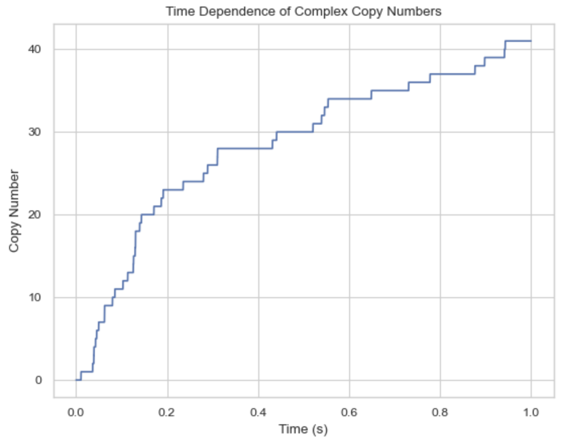
Analyze the NERDSS outputs
Time (s): 0
50  A: 1.
50  B: 1.
50  C: 1.
Time (s): 0.0001
50  A: 1.
50  B: 1.
50  C: 1.
Time (s): 0.0002
50  A: 1.
50  B: 1.
50  C: 1.

...

Time (s): 0.9999
41  A: 1. B: 1. C: 1.
5   A: 1. C: 1.
4   B: 1. C: 1.
4   A: 1. B: 1.
1   B: 1.
Time (s): 1
41  A: 1. B: 1. C: 1.
5   A: 1. C: 1.
4   B: 1. C: 1.
4   A: 1. B: 1.
1   B: 1.
import ioNERDSS as ion


filename = './histogram_complexes_time.dat'
desired_components = ["A: 1", "B: 1", "C: 1"]
times, counts = ion.get_time_dependence(filename, desired_components)
ion.plot_time_dependence(times, counts)